About `coordinate systems and affines` in Nibabel

There are many continuously updated Python libraries that can be used or specialized for Medical Imaging, such as, SimpleITK, NiBabel, scikit-image, etc. Each medical imaging tool has its own internal data structure, but they all serve real-world people of interest. Therefore, when interacting with people, each of these tools is bound to exhibit characteristics that are independent of its own data structure and only relevant to the real world items.

In this article, we are around coordinate systems and affines of nibabel and we mainly record some universal concepts, technologies, and terminologies about medical images, especially MRI images (Nifity format). These records may be also useful when dealing with other formats, other types of medical images, or when using other medical imaging tools.

Most of the conceptual content blocks in this article are excerpts from nibabel‘s official documents. These content blocks may be scattered throughout this article but are all appended with marked annotations (footnotes), even though they are from the same document/webpage. This may lead to repetitive annotations, and annoying readers, but it is a respect for copyright.

Precedent Concepts and Analysis

nibabel image：A nibabel image object is the association of three things:¹
- an N-D array containing the image data;
- a (4, 4) affine matrix mapping array coordinates to coordinates in some RAS+ world coordinate space (Coordinate systems and affines);
- image metadata in the form of a header.
grayscale: graded between black for the minimum value, white for the maximum²
voxel: a voxel is a pixel with volume.³ If a 2D image represents a slice from a 3D image with a certain thickness, then each pixel in the slice grayscale image also represents a voxel. A 3D array is therefore also a voxel array.
voxel coordinates: A voxel coordinate is a coordinate into a voxel array. A coordinate is a set of numbers giving positions relative to a set of axes on an image data array. A voxel coordinate tells us almost nothing about where the data came from in terms of position in the scanner. This is because the scanner allows us to collect voxel data in almost any arbitrary position and orientation within the magnet. ⁴ If we collect a new data from a different field of view and orientation, we will get an image that cannot be related to the original image easily by voxel coordinates.
reference space: To be able to easily relate the data from different field of view and orientations, reference space is introduced. We keep track of the relationship of voxel coordinates to some reference space. In particular, the affine array stores the relationship between voxel coordinates in the image data array and coordinates in the reference space. ⁵ If we know the relationship of (voxel coordinates to the reference space) for both images, we can use this information to relate voxel coordinates of them.
scanner-subject reference space: The space in “reference space” means an item that defined by an ordered set of axes. For our 3D spatial world, it is a set of 3 independent axes. We can decide what space we want to use, by choosing these axes. We need to choose the origin(原点) of the axes, their direction and their units. ⁶A set of three orthogonal(正交) scanner axes can be described as:
- The origin of the axes is at the magnet isocenter. This is coordinate (0, 0, 0) in our reference space. All three axes pass through the isocenter.
- The units for all three axes are millimeters.
- Imagine an observer standing behind the scanner looking through the magnet bore towards the end of the scanner bed. Imagine a line traveling towards the observer through the center of the magnet bore, parallel to the bed, with the zero point at the magnet isocenter, and positive values closer to the observer. Call this line the scanner-bore axis.
- Draw a line traveling from the scanner room floor up through the magnet isocenter towards the ceiling, at right angles to the scanner bore axis. 0 is at isocenter and positive values are towards the ceiling. Call this the scanner-floor/ceiling axis.
- Draw a line at right angles to the other two lines, traveling from the observer’s left, parallel to the floor, and through the magnet isocenter to the observer’s right. 0 is at isocenter and positive values are to the right. Call this the scanner-left/right.
If we make the axes have order (scanner left-right; scanner floor-ceiling; scanner bore) then we have an ordered set of 3 axes and therefore the definition of a 3D space. Call the first axis the “X” axis, the second “Y” and the third “Z”. This reference space is sometimes known as “scanner XYZ”. It was the standard reference space for the predecessor to DICOM, called ACR / NEMA 2.0. If a subject is lying in the usual position for a brain scan, face up and head first in the scanner, then scanner-left/right is also the left-right axis of the subject’s head, scanner-floor/ceiling is the posterior-anterior axis of the head and scanner-bore is the inferior-superior axis of the head.⁷See the diagram below, where the blue circle is the indication of the scanner’s magnet bore:

Sometimes the subject is not lying in the standard position. For example, the subject may be lying with their face pointing to the right (in terms of the scanner-left/right axis). In that case “scanner XYZ” will not tell us about the subject’s left and right, but only the scanner‘s left and right. We might prefer to know where we are in terms of the subject’s left and right.⁸

To deal with this problem, most reference spaces use subject- or patient- centered scanner coordinate systems. In these systems, the axes are still the scanner axes above, but the ordering and direction of the axes come from the position of the subject. The most common subject-centered scanner coordinate system in neuroimaging is called “scanner RAS” (right, anterior, superior). Here the scanner axes are reordered and flipped so that the first axis is the scanner axis that is closest to the left-to-right axis of the subject, the second is the closest scanner axis to the posterior-anterior axis of the subject, and the third is the closest scanner axis to the inferior-superior axis of the subject. For example, if the subject was lying face to the right in the scanner, then the first (X) axis of the reference system would be scanner-floor/ceiling, but reversed so that positive values are towards the floor. This axis goes from left to right in the subject, with positive values to the right. The second (Y) axis would be scanner-left/right (posterior-anterior in the subject), and the Z axis would be scanner-bore (inferior-superior).⁹See the diagram below, where the blue circle is the indication of the scanner’s magnet bore:

Reading names of reference spaces can be confusing because of different meanings that authors use for the same terms, such as ‘left’ and ‘right’. We are using the term “RAS” to mean that the axes are (in terms of the subject): left to Right; posterior to Anterior; and inferior to Superior, respectively. Although it is common to call this convention “RAS”, it is not quite universal, because some use “R”, “A” and “S” in “RAS” to mean that the axes starts on the right, anterior, superior of the subject, rather than ending on the right, anterior, superior. In other words, they would use “RAS” to refer to a coordinate system we would call “LPI”. To be safe, we’ll call our interpretation of the RAS convention “RAS+”, meaning that Right, Anterior, Superior are all positive values on these axes.¹⁰

Some people also use “right” to mean the right hand side when an observer looks at the front of the scanner, from the foot the scanner bed. Unfortunately, this means that you have to read coordinate system definitions carefully if you are not familiar with a particular convention. We nibabel / nipy folks agree with most of our brain imaging friends and many of our enemies in that we always use “right” to mean the subject’s right.¹¹
voxel space: Voxel coordinates are also in a space. In this case the space is defined by the three voxel axes (first axis, second axis, third axis), where 0, 0, 0 is the center of the first voxel in the array and the units on the axes are voxels. Voxel coordinates are therefore defined in a reference space called voxel space.¹²
affine matrix: Describe (encode) a group of linear/affine transformations, including translations, rotations and zooms, for coordinates transform. For example, we have voxel coordinates (in voxel space) and we want to get scanner RAS+ coordinates corresponding to the voxel coordinates. Then, we need a coordinate transform (affine matrix) to take us from voxel coordinates to scanner RAS+ coordinates. ¹³ This affine array has another pleasant property — is usually invertible. So, the inverse of this affine matrix gives the mapping from scanner to voxel. That means that the inverse of the affine matrix gives the transformation from scanner RAS+ coordinates to voxel coordinates in the image data.

Consider we have a affine array \(A\) for img_a, and affine array \(B\) for img_b. \(A\) gives the mapping from voxels in the image data array of img_a to millimeters in scanner RAS+. \(B\) gives the mapping from voxels in the image data array of img_b to millimeters in scanner RAS+. Now let’s say we have a particular voxel coordinate \((i,j,k)\) in the data array of img_a and we want to find the voxel in img_b that is in the same spatial position. Call this matching voxel coordinate \((i^{'},j^{'},k^{'})\). We first apply the transform from img_a voxels to scanner RAS+ (\(A\)) and then apply the transform from scanner RAS+ to voxels in someones_anatomy.nii.gz (\(B^{-1}\)): \[ \begin{bmatrix} i^{'} \\ j^{'} \\ k^{'} \\ 1 \\ \end{bmatrix}=B^{-1}A\begin{bmatrix} i \\ j \\ k \\ 1 \\ \end{bmatrix} \]
other reference spaces:
- MNI reference space (MNI RAS+ space): describe the voxel locations relate to a template brain, the Montreal Neurological Institute (MNI) template brain:
  - The origin (0, 0, 0) point is defined to be the point that the anterior commissure of the MNI template brain crosses the midline (the AC point).
  - Axis units are millimeters.
  - The Y axis follows the midline of the MNI brain between the left and right hemispheres, going from posterior (negative) to anterior (positive), passing through the AC point. The template defines this line.
  - The Z axis is at right angles to the Y axis, going from inferior (negative) to superior (positive), with the superior part of the line passing between the two hemispheres.
  - The X axis is a line going from the left side of the brain (negative) to right side of the brain (positive), passing through the AC point, and at right angles to the Y and Z axes.
- Talairach RAS+ space: To align an image to the Talairach atlas brain. This brain has a different shape and size than the MNI brain. The origin is the AC point, but the Y axis passes through the point that the posterior commissure crosses the midline (the PC point), giving a slightly different trajectory from the MNI Y axis. Like the MNI RAS+ space, the Talairach axes also run left to right, posterior to anterior and inferior superior, so this is the Talairach RAS+ space.¹⁴
- LPS+ space: DICOM files map input voxel coordinates to coordinates in scanner LPS+ space. Scanner LPS+ space uses the same scanner axes and isocenter as scanner RAS+, but the X axis goes from right to the subject’s Left, the Y axis goes from anterior to Posterior, and the Z axis goes from inferior to Superior. A positive X coordinate in this space would mean the point was to the subject’s left compared to the magnet isocenter.¹⁵
nibabel’s conventional practice: Nibabel images always use RAS+ output coordinates, regardless of the preferred output coordinates of the underlying format. Convention that output with RAS+ coordinates is the most popular in neuroimaging; for example, it is the standard used by NIfTI and MINC formats. Nibabel does not enforce a particular RAS+ space. For example, NIfTI images contain codes that specify whether the affine maps to scanner or MNI or Talairach RAS+ space. For the moment, one has to consult the specifics of each format to find which RAS+ space the affine maps to.
radiological vs neurological conventions:
- radiological convention: Radiologists like looking at their images with the patient’s left on the right of the image. If they are looking at a brain image, it is as if they were looking at the brain slice from the point of view of the patient’s feet. ¹⁶
- neurological convention: Neurologists like looking at brain images with the patient’s right on the right of the image. This perspective is as if the neurologist is looking at the slice from the top of the patient’s head. ¹⁷
The convention is one of image display. The image can have any voxel arrangement on disk or memory, and any output reference space; it is only necessary for the software displaying the image to know the reference space and the (probably affine) mapping between voxel space and reference space; then the software can work out which voxels are on the left or right of the subject and flip the images to the taste of the viewer. We could unpack these uses as neurological display convention and radiological display convention.¹⁸ The following is a graphic by Chris Rorden showing these display conventions, where the 3D rendering behind the sections shows the directions that the neurologist and radiologist are thinking of, and the subject has a stroke in left temporal lobe, causing a dark area on the MRI: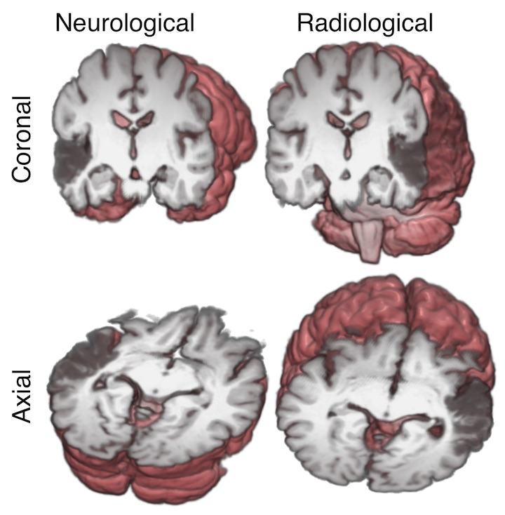

To conclude the above concepts, a nibabel image uses affine to describe the relationship between its original data structure to a conventional space of real-world. If we fully understand the concepts of reference spaces and affine, we will establish the bridge in our mind span real-world subjects and medical imaging tools’ data structures. Then, the last thing left is about how to use high-level APIs supported by these medical imaging tools to realize our targets. The point is, we can just consider ourselves as normal real-world users (no matter how we are acquainted with computer science), and use high-level APIs as much as possible instead of low-level APIs directly related to those internal data structures, thereby improving efficiency. The following sections will post some useful operations with nibabel and more details.

Some operations with nibabel

Let’s divide these operations into 3 parts, i.e., “read”, “save” and “process”.

read

load(). Refer to Nibabel images:

import os
import numpy as np
from nibabel.testing import data_path
example_filename = os.path.join(data_path, 'example4d.nii.gz')
import nibabel as nib
img = nib.load(example_filename)
print(type(img))
# <class 'nibabel.nifti1.Nifti1Image'>

Get dataobj, affine and header. Here voxel data is in dataobj and meta info is in header. And, affine is just from meta info but set as a fast attribute by nibabel for us to use. Refer to Nibabel images:

print(img.dataobj)
# <nibabel.arrayproxy.ArrayProxy object at 0x7f8fed4c6990>
print(img.affine)
# [[-2.00000000e+00  6.71471565e-19  9.08102451e-18  1.17855103e+02]
#  [-6.71471565e-19  1.97371149e+00 -3.55528235e-01 -3.57229424e+01]
#  [ 8.25548089e-18  3.23207617e-01  2.17108178e+00 -7.24879837e+00]
#  [ 0.00000000e+00  0.00000000e+00  0.00000000e+00  1.00000000e+00]]
print(img.header)
# <class 'nibabel.nifti1.Nifti1Header'> object, endian='<'
# sizeof_hdr      : 348
# data_type       : b''
# db_name         : b''
# extents         : 0
# session_error   : 0
# regular         : b'r'
# dim_info        : 57
# dim             : [  4 128  96  24   2   1   1   1]
# intent_p1       : 0.0
# intent_p2       : 0.0
# intent_p3       : 0.0
# intent_code     : none
# datatype        : int16
# bitpix          : 16
# slice_start     : 0
# pixdim          : [-1.000000e+00  2.000000e+00  2.000000e+00  2.199999e+00  2.000000e+03
#   1.000000e+00  1.000000e+00  1.000000e+00]
# vox_offset      : 0.0
# scl_slope       : nan
# scl_inter       : nan
# slice_end       : 23
# slice_code      : unknown
# xyzt_units      : 10
# cal_max         : 1162.0
# cal_min         : 0.0
# slice_duration  : 0.0
# toffset         : 0.0
# glmax           : 0
# glmin           : 0
# descrip         : b'FSL3.3\x00 v2.25 NIfTI-1 Single file format'
# aux_file        : b''
# qform_code      : scanner
# sform_code      : scanner
# quatern_b       : -1.9451068e-26
# quatern_c       : -0.9967085
# quatern_d       : -0.08106874
# qoffset_x       : 117.8551
# qoffset_y       : -35.722942
# qoffset_z       : -7.2487984
# srow_x          : [-2.0000000e+00  6.7147157e-19  9.0810245e-18  1.1785510e+02]
# srow_y          : [-6.7147157e-19  1.9737115e+00 -3.5552824e-01 -3.5722942e+01]
# srow_z          : [ 8.2554809e-18  3.2320762e-01  2.1710818e+00 -7.2487984e+00]
# intent_name     : b''
# magic           : b'n+1'

Get voxel data by get_fdata() or low-level dataobj[...]. Here get_fdata() will cast voxel data into np.float64 dtype automatically by default. So, if we wang to get original voxel data with original dtype , an officially recommended method np.asanyarray() may be needed. Otherwise, we should use low-level dataobj[...]. Refer to Nibabel images:

print(img.get_fdata().shape,img.get_fdata().dtype)
# (128, 96, 24, 2) float64
print(np.asanyarray(img.dataobj).shape,np.asanyarray(img.dataobj).dtype)
# (128, 96, 24, 2) int16
print(np.asarray(img.dataobj).shape,np.asarray(img.dataobj).dtype)
# (128, 96, 24, 2) int16
print(img.dataobj[...].shape,img.dataobj[...].dtype)
# (128, 96, 24, 2) int16

Get some meta info from header, such as get_data_shape(), get_data_dtype(), get_zooms() and get_xyzt_units(). Refer to Nibabel images:

print(img.header.get_data_shape())
# (128, 96, 24, 2)
print(img.header.get_data_dtype())
# int16
print(img.header.get_zooms())
# (2.0, 2.0, 2.199999, 2000.0)
print(img.header.get_xyzt_units())
# ('mm', 'sec')

About array proxy and caching. Refer to Images and memory:

We saw in Nibabel images that images loaded from disk are usually proxy images. Proxy images are images that have a dataobj property that is not a numpy array, but an array proxy that can fetch the array data from disk. We also saw in Proxies and caching that get_fdata() will (by default) load the array data into an internal image cache. The image returns the cached copy on the next call to get_fdata():¹⁹

import os
import numpy as np
from nibabel.testing import data_path
example_file = os.path.join(data_path, 'example4d.nii.gz')
import nibabel as nib
img = nib.load(example_file)
data = img.get_fdata()
data_again = img.get_fdata()
assert data_again is data

Check state of cache by in_memory and use uncache() to release(empty) cache. Modify on the data fromget_fdata() is just modify the cached data but not the original data.

array_data = np.arange(24, dtype=np.int16).reshape((2, 3, 4))
affine = np.diag([1, 2, 3, 1])
array_img = nib.Nifti1Image(array_data, affine)
assert array_img.in_memory
img = nib.load(example_file)
assert not img.in_memory
data = img.get_fdata()
assert img.in_memory
img.uncache()
assert not img.in_memory
data_again = img.get_fdata()
assert not (data_again is data)

data = img.get_fdata() 
print(data[0, 0, 0, 0])
# 0.0
data[0, 0, 0, 0] = 99
assert img.get_fdata()[0, 0, 0, 0]==99
img.uncache()
assert img.get_fdata()[0, 0, 0, 0]==0

To avoid caching, use np.asarray from dataobj directly or use caching keyword of get_fdata().

proxy_img = nib.load(example_file)
data_array = np.asarray(proxy_img.dataobj)
print(type(data_array))
# <class 'numpy.ndarray'>

proxy_img = nib.load(example_file)
data = proxy_img.get_fdata(caching='unchanged')
assert not proxy_img.in_memory
data = proxy_img.get_fdata(caching='fill')
assert proxy_img.in_memory
# caching='unchanged' will leave the cache full if it is already full.
data = proxy_img.get_fdata(caching='unchanged')
assert proxy_img.in_memory

To slice, array proxy can usually save time and memory if we do not need whole data.

proxy_img = nib.load(example_file)
vol1 = proxy_img.dataobj[..., 1]
print(vol1.shape)
# (128, 96, 24)

save

Create from scratch. A new nib.Nifti1Image image needs at least voxel array and affine to initialize. Refer to Nibabel images:

array_data = np.arange(24, dtype=np.int16).reshape((2, 3, 4))
affine = np.diag([1, 2, 3, 1])
array_img = nib.Nifti1Image(array_data, affine)
print(array_img.dataobj)
# [[[ 0  1  2  3]
#   [ 4  5  6  7]
#   [ 8  9 10 11]]

#  [[12 13 14 15]
#   [16 17 18 19]
#   [20 21 22 23]]]

save() or to_filename(). And, get_filename() and set_filename() may be also useful. Refer to Nibabel images:

import tempfile
with tempfile.NamedTemporaryFile(suffix='.nii.gz') as fp:
    nib.save(array_img, fp.name)
    img = nib.load(fp.name)
    print(type(img))
# <class 'nibabel.nifti1.Nifti1Image'>

with tempfile.NamedTemporaryFile(suffix='.nii.gz') as fp:
    array_img.to_filename(fp.name) 
    img = nib.load(fp.name)
    print(type(img))
# <class 'nibabel.nifti1.Nifti1Image'>
img.set_filename('another_image.nii')
print(img.get_filename())
# another_image.nii

about files: If an image can be loaded or saved on disk, the image will have an attribute called file_map. The img.file_map is a dictionary where the keys are the names of the files that the image uses to load / save on disk, and the values are FileHolder objects, that usually contain the filenames that the image has been loaded from or saved to.²⁰ Different formats of images need different numbers of files to make up the whole. Refer to Nibabel images:

array_data = np.arange(24, dtype=np.int16).reshape((2, 3, 4))
affine = np.diag([1, 2, 3, 1])
import tempfile
with tempfile.NamedTemporaryFile(suffix='.nii.gz') as fp:
    array_img = nib.Nifti1Image(array_data, affine)
    nib.save(array_img, fp.name)
    img_again = nib.load(fp.name)
    print(list(img_again.file_map))
    # ['image']
    print(img_again.file_map['image'].filename)
    # /tmp/tmphm7_zeoh.nii.gz
with tempfile.NamedTemporaryFile(suffix='.img') as fp:    
    pair_img = nib.Nifti1Pair(array_data, np.eye(4))
    nib.save(pair_img, fp.name)
    pair_img = nib.load(fp.name)
    print(sorted(pair_img.file_map))
    # ['header', 'image']
    print(pair_img.file_map['header'].filename)
    # /tmp/tmpbqnu65ff.hdr
    print(pair_img.file_map['image'].filename)
    # /tmp/tmpbqnu65ff.img
with tempfile.NamedTemporaryFile(suffix='.img') as fp:    
    ana_img = nib.AnalyzeImage(array_data, np.eye(4))
    nib.save(ana_img, fp.name)
    ana_img = nib.load(fp.name)
    print(sorted(ana_img .file_map))
    # ['header', 'image', 'mat']
    print(ana_img.file_map['header'].filename)
    # /tmp/tmpb2u21kbl.hdr
    print(ana_img.file_map['image'].filename)   
    # /tmp/tmpb2u21kbl.img
    print(ana_img.file_map['mat'].filename)  
    # /tmp/tmpb2u21kbl.mat

process

slicer. The slicer attribute provides an array-slicing interface to produce new images with an appropriately adjusted header, such that the data at a given RAS+ location is unchanged.²¹ The basic syntax is consistent with Python and Nnumpy slice. Slicer can work with array proxy to save both time and memory. From Saving time and memory, img.dataobj[...] can also be a slicing method with array proxy. Refer to Nibabel images:

import os
import numpy as np
from nibabel.testing import data_path
example_filename = os.path.join(data_path, 'example4d.nii.gz')
import nibabel as nib
img = nib.load(example_filename)
cropped_img = img.slicer[32:-32, ...]
print(cropped_img.shape)
# (64, 96, 24, 2)
# 
np.testing.assert_array_equal(cropped_img.get_fdata(), img.dataobj[32:-32, ...]) 
np.testing.assert_array_equal(cropped_img.get_fdata(), img.get_fdata()[32:-32, ...])
# the image affine was adjusted so that the X-translation is 32 voxels (64mm) less:
print(img.affine - cropped_img.affine)
# [[ 0.  0.  0. 64.]
#  [ 0.  0.  0.  0.]
#  [ 0.  0.  0.  0.]
#  [ 0.  0.  0.  0.]]

Get orientations by nib.orientations.aff2axcodes, and rearrange the image voxel axes to make them as close as possible to RAS+ orientation by as_closest_canonical. We refer to this voxel orientation as canonical voxel orientation, because RAS+ is our canonical world orientation. Rearranging the voxel axes means reversing and / or reordering the voxel axes. ²² Refer to Nibabel images, and Image voxel orientation:

print(nib.orientations.aff2axcodes(img.affine))
# ('L', 'A', 'S')
print(nib.orientations.aff2axcodes(img.slicer[::-1].affine))
# ('R', 'A', 'S')
print(nib.orientations.aff2axcodes((new_img:=img.slicer[32:-32, ...].slicer[::-1]).affine))
# ('R', 'A', 'S')
print(new_img.affine)
# [[ 2.00000000e+00  6.71471565e-19  9.08102451e-18  5.38551025e+01]
#  [ 6.71471565e-19  1.97371149e+00 -3.55528235e-01 -3.57229424e+01]
#  [-8.25548089e-18  3.23207617e-01  2.17108178e+00 -7.24879837e+00]
#  [ 0.00000000e+00  0.00000000e+00  0.00000000e+00  1.00000000e+00]]

img = nib.load(example_filename)
canonical_img = nib.as_closest_canonical(img)
print(canonical_img.affine)
# [[ 2.00000000e+00  6.71471565e-19  9.08102451e-18 -1.36144897e+02]
#  [ 6.71471565e-19  1.97371149e+00 -3.55528235e-01 -3.57229424e+01]
#  [-8.25548089e-18  3.23207617e-01  2.17108178e+00 -7.24879837e+00]
#  [ 0.00000000e+00  0.00000000e+00  0.00000000e+00  1.00000000e+00]]
print(nib.aff2axcodes(canonical_img.affine))
# ('R', 'A', 'S')

To show picture, use matplotlib.pyplot where the keyword origin="lower" in imshow() is import. Because by this keyword, we do not need to care about the mapping rules that from voxel space or RAS+ space to pyplot’s image space. (imshow() on screen takes a default rule that the X axis is from the left to the right while the Y axis is from the top to the button, which will lead to inversed slice images against our standard convention when output if origin="higher" or not set.) Refer to Nibabel images.

import os
import numpy as np
from nibabel.testing import data_path
example_filename = os.path.join(data_path, 'example4d.nii.gz')
import nibabel as nib
img = nib.as_closest_canonical(nib.load(example_filename))
print(nib.aff2axcodes(img.affine)) 
# ('R', 'A', 'S')                   
img_data = img.get_fdata()
print(img_data.shape)
# (128, 96, 24, 2)
import matplotlib.pyplot as plt
def show_slices(slices):
   """ Function to display row of image slices """
   fig, axes = plt.subplots(1, len(slices))
   for i, slice in enumerate(slices):
       axes[i].imshow(slice.T, cmap="gray", origin="lower")
slice_0 = img_data[64, :, :,0]
slice_1 = img_data[:, 48, :,0]
slice_2 = img_data[:, :, 12,0]
show_slices([slice_0, slice_1, slice_2])
plt.suptitle("Center slices for example image")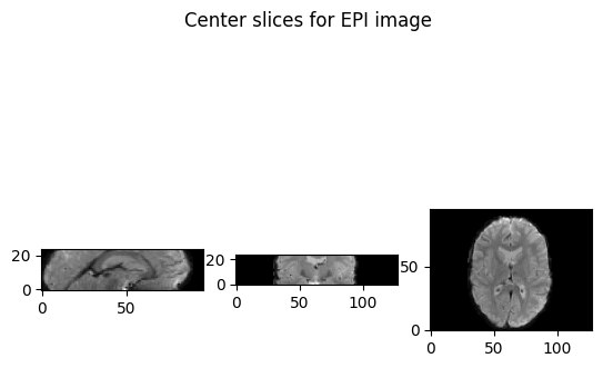

Appendix (To be extended)

Nifty data format(structure)
- History
- Meaning of each item
- Names of each item in Chinese (with references)
- …
Dicom data format(structure)
- History
- Meaning of each item
- Names of each item in Chinese (with references)
- …
Some key docs:

(2023, March 29). Nibabel images — NiBabel 5.0.0 documentation. Nipy. https://nipy.org/nibabel/nibabel_images.htmlms.html ↩︎
(2023, March 29). Neuroimaging in Python — NiBabel 5.0.0 documentation. Nipy. https://nipy.org/nibabel/coordinate_systems.html ↩︎
(2023, March 29). Neuroimaging in Python — NiBabel 5.0.0 documentation. Nipy. https://nipy.org/nibabel/coordinate_systems.html ↩︎
(2023, March 29). Neuroimaging in Python — NiBabel 5.0.0 documentation. Nipy. https://nipy.org/nibabel/coordinate_systems.html ↩︎
(2023, March 29). Neuroimaging in Python — NiBabel 5.0.0 documentation. Nipy. https://nipy.org/nibabel/coordinate_systems.html ↩︎
(2023, March 29). Neuroimaging in Python — NiBabel 5.0.0 documentation. Nipy. https://nipy.org/nibabel/coordinate_systems.html ↩︎
(2023, March 29). Neuroimaging in Python — NiBabel 5.0.0 documentation. Nipy. https://nipy.org/nibabel/coordinate_systems.html ↩︎
(2023, March 29). Neuroimaging in Python — NiBabel 5.0.0 documentation. Nipy. https://nipy.org/nibabel/coordinate_systems.html ↩︎
(2023, March 29). Neuroimaging in Python — NiBabel 5.0.0 documentation. Nipy. https://nipy.org/nibabel/coordinate_systems.html ↩︎
(2023, March 29). Neuroimaging in Python — NiBabel 5.0.0 documentation. Nipy. https://nipy.org/nibabel/coordinate_systems.html ↩︎
(2023, March 29). Neuroimaging in Python — NiBabel 5.0.0 documentation. Nipy. https://nipy.org/nibabel/coordinate_systems.html ↩︎
(2023, March 29). Neuroimaging in Python — NiBabel 5.0.0 documentation. Nipy. https://nipy.org/nibabel/coordinate_systems.html ↩︎
(2023, March 29). Neuroimaging in Python — NiBabel 5.0.0 documentation. Nipy. https://nipy.org/nibabel/coordinate_systems.html ↩︎
(2023, March 29). Neuroimaging in Python — NiBabel 5.0.0 documentation. Nipy. https://nipy.org/nibabel/coordinate_systems.html ↩︎
(2023, March 29). Neuroimaging in Python — NiBabel 5.0.0 documentation. Nipy. https://nipy.org/nibabel/coordinate_systems.html ↩︎
(2023, March 30). Neuroimaging in Python — NiBabel 5.0.0 documentation. Nipy. https://nipy.org/nibabel/neuro_radio_conventions.html ↩︎
(2023, March 30). Neuroimaging in Python — NiBabel 5.0.0 documentation. Nipy. https://nipy.org/nibabel/neuro_radio_conventions.html ↩︎
(2023, March 30). Neuroimaging in Python — NiBabel 5.0.0 documentation. Nipy. https://nipy.org/nibabel/neuro_radio_conventions.html ↩︎
(2023, March 31). Neuroimaging in Python — NiBabel 5.0.0 documentation. Nipy. https://nipy.org/nibabel/images_and_memory.html ↩︎
(2023, March 29). Nibabel images — NiBabel 5.0.0 documentation. Nipy. https://nipy.org/nibabel/nibabel_images.htmlms.html ↩︎
(2023, March 29). Nibabel images — NiBabel 5.0.0 documentation. Nipy. https://nipy.org/nibabel/nibabel_images.htmlms.html ↩︎
(2023, March 31). Neuroimaging in Python — NiBabel 5.0.0 documentation. Nipy. https://nipy.org/nibabel/image_orientation.html ↩︎